HISTORICAL TRAJECTORY GUIDANCE

TGuide

Faster Autoregressive Video Diffusion
via Historical Trajectory Guidance

Use historical trajectories to guide current predictions.

Accelerating four-step video generation with a lightweight,
history-guided predictor — while preserving generation quality.

Explore demos Read the paper

Anonymous authors · Under double-blind review

1.89×

Denoising speedup

Self Forcing · 333 frames

+0.16

VBench total score

vs. the original 4-step model

81 → 333

Train short. Generate longer.

Training frames → evaluation frames

THE IDEA

Historical trajectories guide
the current prediction.

Few-step distillation makes video diffusion faster, but each remaining step still runs a full diffusion transformer. Simply reusing features becomes unreliable when denoising steps are far apart.

TGuide looks across video chunks. The previous chunk’s features at the same denoising timestep provide a complementary reference. Our Anchor–Transport–Correct predictor retrieves and adapts this history to replace selected full-model evaluations.

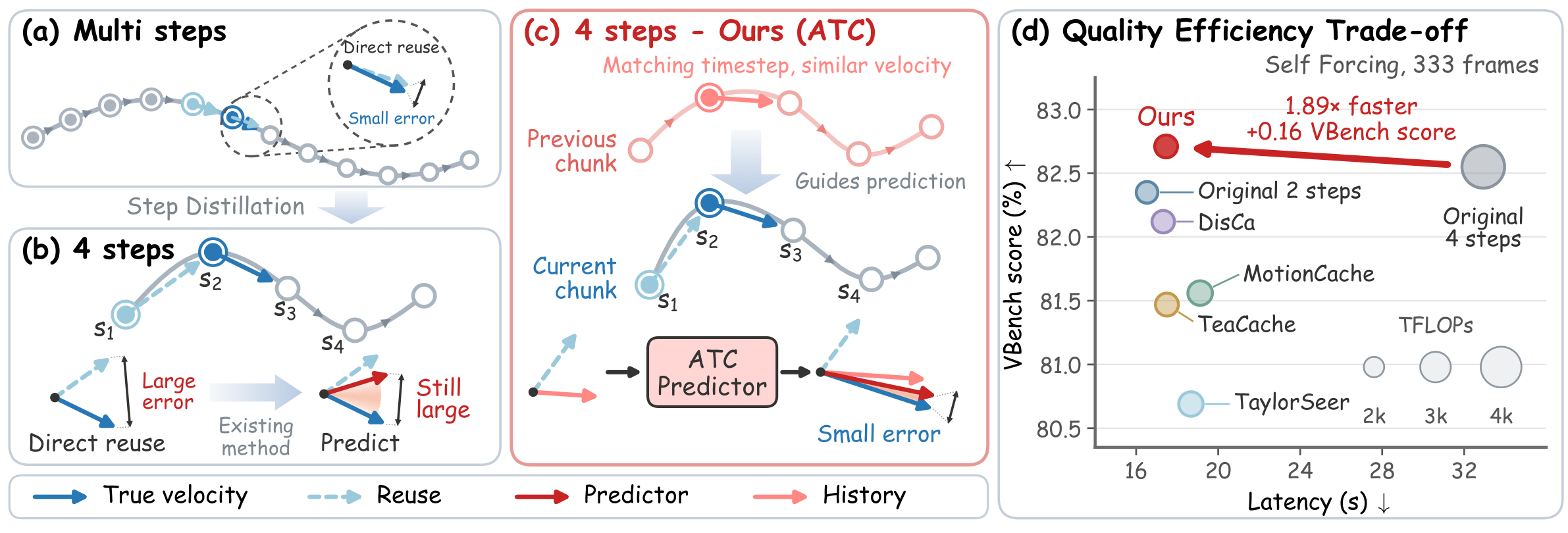
Figure 1. Many-step sampling permits nearby velocity reuse, but four-step sampling introduces large reuse and prediction errors. TGuide combines the current chunk’s earlier-step features with the previous chunk’s same-timestep features to reduce prediction error. The quality–efficiency plot shows a 1.89× denoising speedup and a 0.16-point VBench improvement on Self Forcing at 333 frames. — **Match the denoising stage. Retrieve across chunks.** Historical features at the target timestep complement the current chunk’s earlier-step features, guiding more accurate prediction even when only four denoising steps remain.

SEE IT IN MOTION

Less computation.
More of the detail that matters.

Explore 20 side-by-side comparisons across two autoregressive generators.

Case 08

Self Forcing

TGuide (Ours) appears in the top-left panel.

Comparison clips, including their prompts and method labels. Playback shows generated content; the speedup labels refer to generation latency.

HOW IT WORKS

Start with the current chunk.
Refine it with history.

Anchor and Transport provide complementary information. Correct combines them into one hidden-state prediction.

What information is already available?

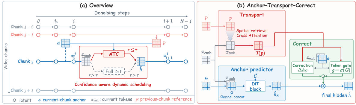
At denoising step $i$ of video chunk $j$ , ATC uses two cached hidden states. A hidden state is the diffusion transformer’s internal feature representation, before its output head converts it into a denoising velocity.

CURRENT CHUNK · EARLIER STEP

a=h_{i_a}^{j}

The anchor $a$ preserves the current chunk’s spatial layout, but comes from an earlier denoising stage ( $i_a<i$ , usually $i_a=i-1$ ).

PREVIOUS CHUNK · SAME STEP

p=h_i^{j-1}

The historical reference $p$ is already at the target denoising stage, but motion may have shifted its content to different spatial positions.

The predictor also receives $x_{\mathrm{emb}}$ , the current noisy latent after the input head, and $\mathcal C$ , the generation conditions and historical key–value (KV) context.

01 / ANCHOR

Predict how the current features should change.

Starting from $a$ , a lightweight predictor uses the current noisy tokens $x_{\mathrm{emb}}$ and context $\mathcal C$ to estimate the change needed to reach the target denoising stage. Adding this change to $a$ gives the initial prediction $\hat h_A$ .

DENOISING EVOLUTION

\hat h_A = a + \Delta h_D\big(x_{\mathrm{emb}},a,\mathcal C\big)

$\Delta h_D$ is the learned denoising increment. The resulting $\hat h_A$ will be refined in Correct.

02 / TRANSPORT

Find the historical features that match now.

The current noisy tokens query the previous chunk’s reference $p$ through cross-attention. Retrieving across spatial positions accounts for content displaced by motion and produces $\mathcal T(p)$ , history aligned to the current tokens for use in Correct.

SPATIAL RETRIEVAL

\mathcal T(p)=\mathrm{CrossAttn}\!\big(Q(x_{\mathrm{emb}}),K(p),V(p)\big)

$Q$ projects current tokens into queries; $K$ and $V$ project historical features into keys and values. $\mathcal T(p)$ is the retrieved historical state.

03 / CORRECT

Use retrieved history to refine the prediction.

A lightweight network combines $\mathcal T(p)$ with $x_{\mathrm{emb}}$ and $a$ to predict a correction. The learned gate $g$ controls its strength separately for each token. Adding the gated correction to $\hat h_A$ produces the final hidden state $\hat h$ .

GATED HISTORICAL CORRECTION

\hat h=\hat h_A+g\odot\Delta h_C\big(x_{\mathrm{emb}},a,\mathcal T(p)\big)

$\Delta h_C$ predicts the correction; $\odot$ applies each token’s scalar gate across its feature channels. A small gate keeps the result close to $\hat h_A$ .

How is the gate computed?

g=\sigma\!\big(G(x_{\mathrm{emb}},a,\mathcal T(p))\big)

$G$ is a learned gating network and $\sigma$ is the sigmoid function, which bounds each gate between 0 and 1.

TGuide overview: ATC replaces selected full DiT evaluations. Anchor, cross-attention transport, and gated correction combine current features with historical features. — ATC predicts final hidden states, decoded into velocity through the frozen output head. Optional confidence-aware scheduling falls back to the full DiT when estimated risk is high.

TRAINED FOR ITS OWN ROLLOUTS

Learn from the states
you will actually encounter.

Offline regression first teaches ATC to approximate the frozen model. Self-rollout on-policy distillation then adapts it to trajectories shaped by its own predictions, reducing the training–inference gap across both denoising steps and video chunks.

5.3%of a full DiT pass’s FLOPs
ATC on Self Forcing

QUALITY MEETS EFFICIENCY

Faster generation.
A stronger long-horizon result.

Trained on 81 frames. Evaluated up to 333 frames, with the base generator kept frozen.

TGUIDE VS. ORIGINAL 4 STEPS

1.89×

denoising speedup

Original32.93 s

TGuide17.46 s

82.71 VBench total score
+0.16 points over the original model

Self Forcing benchmark results
Method	Latency ↓	Speedup ↑	VBench ↑

Paper, Table 1. Full VBench benchmark; NVIDIA A100; 832 × 480 resolution. Latency measures denoising. TGuide uses the fixed FPPF schedule.

BEYOND TEXT-TO-VIDEO

Camera-conditioned generation, too.

On HY-WorldPlay, TGuide reaches a 1.73× denoising speedup and the best fidelity to the original outputs among the evaluated accelerated methods.

1.73×Speedup

20.52PSNR vs. original

0.1144LPIPS vs. original

Paper, Table 2. HY-WorldPlay, 125 frames. Higher PSNR and lower LPIPS indicate greater fidelity to the original 4-step outputs.

EXPLORE THE FULL WORK

Historical trajectories.
Faster generation.

Architecture, training, ablations, and evaluation protocols.

Read the paper

TGuide

Faster Autoregressive Video Diffusionvia Historical Trajectory Guidance

Historical trajectories guidethe current prediction.

Less computation.More of the detail that matters.

Start with the current chunk.Refine it with history.